|
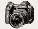
E-510 Image Stabilization How well does it really work? |
|
|
My other articles related to the |
|
One of the most acclaimed new features on the E-510 is the new system of image stabilization. Unfortunately, there is not much known about how effective it may be. The data available on the Web range from anecdotal evidence at best to wishful thinking and numbers taken off the ceiling at worst. This is why I someone had to write this article, and such dirty work usually ends up in my lap. Before continuing, read my general introduction to the subject: Camera Shake and Image Stabilization. That article may contain many things you already know, but also a few you will find new. Experiment design and procedure Now, that you went through the article I've sent you to, you realize that measuring the benefits of an image stabilization system is not a simple thing. For the sake of this report I've developed a statistically sound, unbiased procedure to perform such measurement. The details can be found in a technical article: Measuring the Benefits of Image Stabilization. This may be not a quick read, but understanding what I did is important for the proper interpretation of the results; this is not a simple "five is better than four" affair. Anyway, my procedure boiled down to shooting 200 or more pictures for every focal length tested, reviewing them in a randomized and anonymized way, and assigning the "good", "medium", and "bad" ratings. Instead of describing them, let me show you examples of each (at F=150 mm). |
 Subjective "bad" |
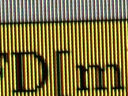 Subjective "medium" |
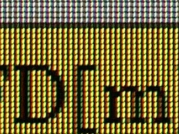 Subjective "good" |
|
For each combination of shutter speed and IS setting (On/Off) a total "success rate" has been computed, based on 20 frames shot, and seen as a single data point in the graphs below. Then, for each focal length tested, these data points were processed numerically to result in just one value, a metrics reflecting how much slower shutter speeds can we use with IS than without. (If you haven't read that article, do it now.) The raw values are listed in Appendix One so those who may be more fluent than I am in data reduction and statistics, can do their own number-crunching their own way. The results Let me show you the results without going through all numbers; the basic results can be found in Appendix Two, if you care. Green points and lines are with image stabilization, yellow ones — without. You may visualize the IS benefit as the distance between the points where both lines cross the 50% level. | |
|
14 mm: IS improves v50 by 1.05 EV (shutter speed factor of 2.06×). The lines behave very nicely, running as parallel as my eye can tell — almost to good to be true (especially at this statistics). I would have called this gain disappointing, if not for the fact that I haven't checked the values of 2-4 EV claimed by some other manufacturers; I suspect that lots of that data comes from imaginative minds of the marketing departments, not from the lab. |
|
|
42 mm: The improvement in v50 is 1.61 EV (3.05×). Interestingly, the value of v0 (0% success rate) improves by about 2.0 EV, while that of v100 (100% good pictures) —by only 1.2 EV. While it is not possible to analytically estimate errors in my coefficients (I would rather have to use a Monte Carlo simulation of the whole experiment, I'm afraid; doable but costly), I believe they can be 0.2 or less; there seems to be some real physics beyond the lines diverging at longer exposures. |
|
|
150 mm: Whoa! v50 improves by 2.23 EV (shutter speeds 4.70× longer), with, again, a stronger effect at the bottom (2.6 EV) than at the top (1.9 EV).
Most probably, a statistical fluctuation is responsible for the dip at stabilized |
|
|
Re-running the measurements for the outlying data point would be plain wrong and dishonest; why not do it many times, stopping only when the stochastic process brings a result satisfying our theories? For my American Readers this may be remindful of the election recount in Florida, or any other similar recount, regardless who calls it. Anyway, that's why I wanted to use some aggregate metrics, based on more than just a few readings. With the stochastic nature of image stabilization, and with subjective evaluation, this is the only chance of getting a meaningful result. One more remark: the image stabilization seems to be doing its best job in preventing a strong camera shake effect at longest focal lengths: not only do the 1/2 s exposures at 42 mm and 150 mm get similar success rates, but the v0 values are almost identical. The inverse proportionality rule to the focal length would let me expect a 1.8 EV difference: log2(150/42); this is well beyond any statistical error. Conclusions First of all, there is no doubt that image stabilization works in the E-510. Secondly, its effects seems to be increasing with the focal length used. It remains unclear if and how it may depend on physical characteristics (mass, size) of the lens. If that dependency is significant, my numerical results will be applicable only to the lenses I've used in the experiment. Third, as the process is based on frequency analysis of the detected camera shake (Olympus says from seven down to below one hertz), its effectiveness will depend on the nature of that shake: various users may see various gains. I think the more savvy ones, knowing how to hold the camera and trip the shutter, may gain less. I'd like to believe I'm in this category, so I wouldn't be surprised to see Aunt Minnie gaining more. Still, I have no evidence to support that theory. Fourth and last: do not understand my reported 1-2 EV benefit as "only" 1-2 EV. Some camera makers may claim 3-4 EV (so does Olympus), but until this is verified using the same measurement method and the same data reduction/interpretation scheme, it is not a meaningful number. The same as "unsurpassed color accuracy" or "mind-boggling detail" (actual quotes from press releases). If someone offers me his/her camera of another brand to put through a 600 frames of torture, I may consider, just for the sake of curiosity, spending a better part of a day to run a similar experiment, even if I have a (long) list of better things to do. This is the end of my little study. What follows is two Appendices, containing the raw data and computed values of my v coefficients — of interest only to a very few Readers. Most probably you will want to ignore them, and justly so. This table show the "bad-medium-good" frame counts for each series of frames, shot at a given focal length and shutter speed combination. Below each triplet of counts, the success rate is shown in percent, i.e., normalized to the 0..100% range. | |
| IS OFF | 1/2" | 1/4" | 1/8" | 1/15" | 1/30" | 1/60" | 1/125" |
|---|---|---|---|---|---|---|---|
| 14 mm | 20-0-0 R = 0 | 16-4-0 R = 10 | 7-4-9 R = 55 | 2-3-15 R = 79.5 | 0-0-20 R = 100 | - | - |
| 42 mm | 20-0-0 R = 0 | 20-0-0 R = 0 | 15-4-1 R = 15 | 9-6-5 R = 40 | 0-4-16 R = 80 | 0-1-19 R = 97.5 | - |
| 150 mm | - | - | 19-1-0 R = 2.5 | 10-10-0 R = 25 | 10-6-4 R = 35 | 4-6-10 R = 65 | 0-0-20 R = 100 |
| IS ON | 1/2" | 1/4" | 1/8" | 1/15" | 1/30" | 1/60" | 1/125" |
| 14 mm | 13-7-0 R = 17.5 | 7-8-5 R = 45 | 1-2-17 R = 80 | 0-0-20 R = 100 | - | - | - |
| 42 mm | 16-3-1 R = 12.5 | 12-3-5 R = 32.5 | 5-5-10 R = 62.5 | 0-0-20 R = 100 | 0-0-20 R = 100 | - | - |
| 150 mm | 16-3-1 R = 12.5 | 12-4-4 R = 30 | 13-3-4 R = 27.5 | 2-2-16 R = 85 | 0-3-17 R = 92.5 | 0-0-20 R = 100 | - |
|
Appendix Two: The v coefficients These are the values of v0 and v100, and v50 in terms of EV as defined in the model description. I'm showing more decimal digits than really needed, so that these values can be used in further calculations. For a better readability, the corresponding shutter speeds (arbitrarily rounded) are shown below. The last column shows the change in v50 due to image stabilization, and the corresponding exposure time increase. |
| IS OFF | IS ON | Δv50 | |||||
|---|---|---|---|---|---|---|---|
| v0 | v100 | v50 | v0 | v100 | v50 | ||
| 14 mm | 1.644 1/3.1" | 4.402 1/21" | 3.023 1/8.1" | .598 1/1.5" | 3.356 1/10" | 1.977 1/3.9" | 1.046 2.06× |
| 42 mm | 2.711 1/6.5" | 5.378 1/42" | 4.045 1/17" | .726 1/1.7" | 4.145 1/18" | 2.436 1/5.4" | 1.609 3.05× |
| 150 mm | 3.294 1/10" | 7.216 1/149" | 5.255 1/38" | .698 1/1.6" | 5.349 1/41" | 3.024 1/8.1" | 2.231 4.70× |
|
|
My other articles related to the |
|
Evolt® and Olympus® are registered trademarks of Olympus Corporation.
This page is not sponsored or endorsed by Olympus (or anyone else) and presents solely the views of the author. |
| Home: wrotniak.net | Search this site | Change font size |
| Posted 2007/08/20; last updated 2009/02/28; touched up 2013/11/01 | Copyright © 2007-2009 by J. Andrzej Wrotniak |